Rebuilding a published study as a tested data pipeline
Rebuilding a published study as a tested data pipeline
OECD regional well-being — 388 regions, 135 indicators, one reproduction
Repository · Read the analysis · Read the robustness study
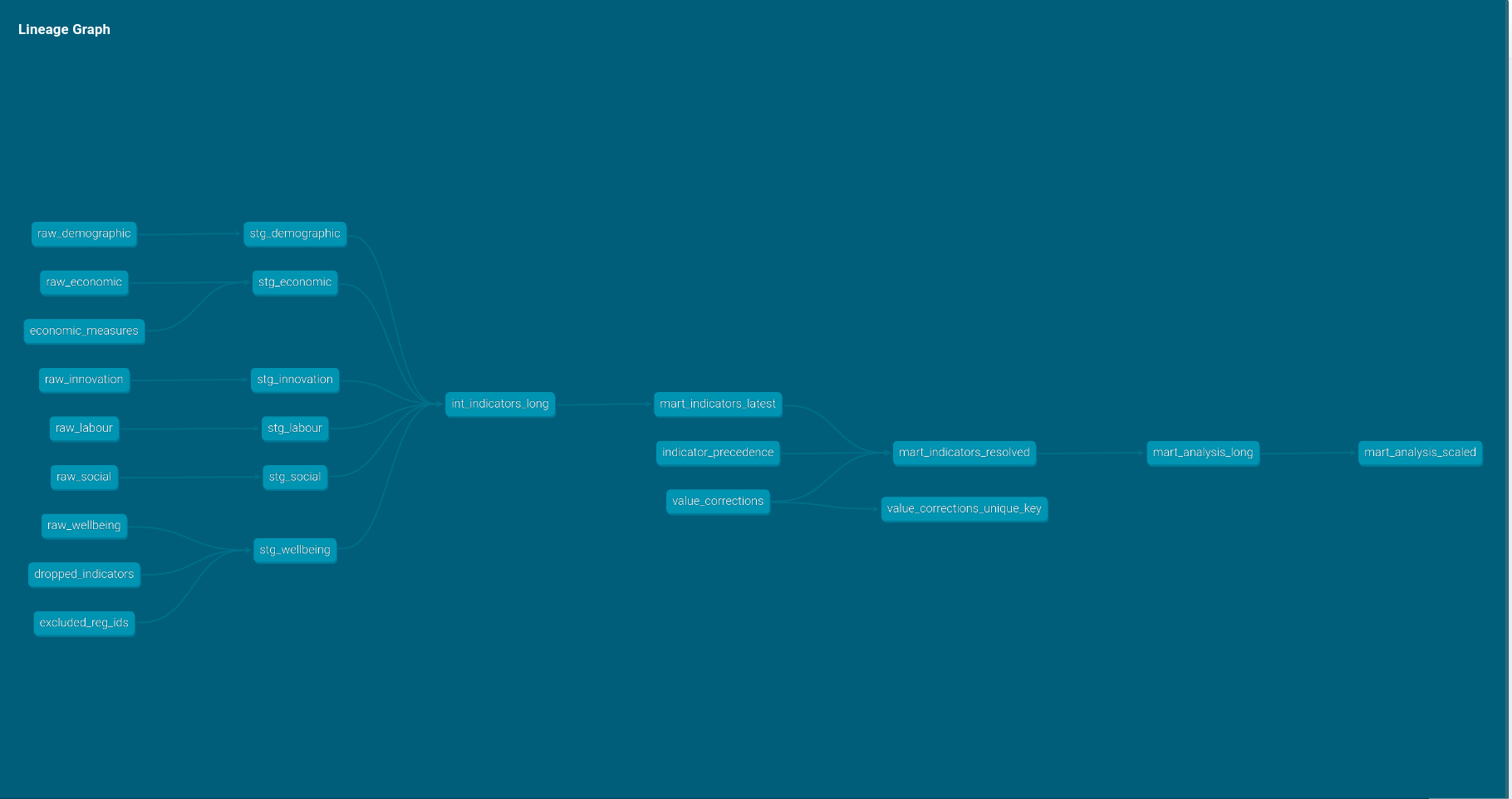
I took the data preparation behind one of my published papers — originally written in R, later ported to pandas — and rebuilt it as a version-controlled, tested pipeline: dbt over DuckDB for the transformations, scikit-learn for the analysis, GitHub Actions running the whole thing in a clean container on every commit.
The output reproduces the published dataset exactly: 388 regions, 135 indicators, every value identical to floating-point precision.
What the tests found
Writing the transformations as tested SQL rather than scripts surfaced four things the original pipeline had resolved silently.
The OECD publishes each series at several territorial levels, and the same region code can carry different values at different levels. Zeeland appears twice with two different waste figures — 71 and 78 — describing genuinely different areas. The original code deduplicated on identifiers while ignoring the values, so which figure survived depended on row order in the source file.
The obvious fix — keep only the larger territorial level — would have silently removed five Estonian regions from the analysis, because Estonia publishes them only at the finer level. No error would have been raised. The rule the pipeline uses now is a preference with a documented fallback.
The list of country codes to exclude turned out to be missing Latvia and Lithuania, which had joined the OECD around the time the data was compiled.
None of this changed the published results. It was found because declarative tests ask precise questions that scripts do not.
Making an implicit design choice explicit
The analysis requires every indicator to be observed for every region, so a single poorly-covered region removes that indicator for all of them. That rule is standard and was applied without examining what it cost.
Sweeping the trade-off shows the cost was substantial and the remedy cheap: dropping the ten worst-covered regions out of 388 — 2.6% of the sample — would have made 44 additional indicators available, a third more than the published analysis used. Almost none of the remaining regions buy anything: the next seventy dropped gain one indicator between them.
Whether that changes any conclusion is the subject of the second document, which runs the full analysis at several points along the trade-off and compares which predictors survive.
Two methods implemented from source
Accumulated Local Effects and Friedman’s H-statistic exist in R’s iml package but have no scikit-learn equivalent. Rather than approximate them, I worked from the R source so the numerical procedure matches — including the parts that are easy to get wrong, such as how empty cells in a two-dimensional grid are filled and how main effects are removed from an interaction surface.
Both are verified against structures with known answers: the interaction surface of an exactly additive model comes out as zero to machine precision, and the surface for a known product recovers that product.
Those checks produced an incidental result worth carrying into the interpretation. A random forest fitted on data with no interaction still reports a substantial one — tree ensembles manufacture structure that is not in the data. This is why the analysis carries two model families through in parallel: agreement between them is what separates a finding from an artefact.
Stack
dbt · DuckDB · SQL · Python · scikit-learn · XGBoost · pandas · pytest · GitHub Actions · Quarto